一、Gaussian_Diffusion.py
1、噪声时间序列:
1
2
3
4
5
6
7
8
9
10
11
12
13
14
15
16
17
| def beta_schedule(schedule_name, num_diffusion_timesteps):
if schedule_name == 'linear':
scale = 1000 / num_diffusion_timesteps
beta_start = scale * 0.0001
beta_end = scale * 0.02
return torch.linspace(beta_start, beta_end, num_diffusion_timesteps, dtype=torch.float64)
elif schedule_name == 'cosine':
s = 0.008
steps = num_diffusion_timesteps + 1
t = torch.linspace(0, num_diffusion_timesteps, steps, dtype=torch.float64)
alphas_cumprod = torch.cos(((t / num_diffusion_timesteps) + s) / (1 + s) * math.pi * 0.5) ** 2
alphas_cumprod = alphas_cumprod / alphas_cumprod[0]
betas = 1 - (alphas_cumprod[1:] / alphas_cumprod[:-1])
return torch.clip(betas, 0, 0.999)
else:
raise ValueError(f"unknown beta schedule{beta_named}, please input linear or cosine")
|
2、GaussianDiffusion类
1)def
init (self,timesteps=1000, beta_name="linear")
1️⃣有关\(\alpha,\beta\)的定义:
🔸\(β_t\):
1
2
| betas = beta_schedule(beta_name, timesteps)
self.betas = betas
|
🔸\(\alpha_t\)(\(\alpha_t = 1 - β_t\)):
1
| self.alphas = 1 - self.betas
|
🔸\(\bar{\alpha}_t\):
1
| self.alphas_cumprod = torch.cumprod(self.alphas, dim=0)
|
🔸\(\bar{\alpha}_{t-1}\):
1
| self.alphas_cumprod_prev = F.pad(self.alphas_cumprod[:-1], (1, 0), value=1.0)
|
2️⃣计算扩散过程\(\textcolor{blue}{q(x_t|x_{t-1})}\)需要的参数:
🔸\(\sqrt{\bar{\alpha}_t}\)
1
| self.sqrt_alphas_cumprod = torch.sqrt(self.alphas_cumprod)
|
🔸\(\sqrt{1-\bar{\alpha}_t}\)
1
| self.sqrt_one_minus_alphas_cumprod = torch.sqrt(1.0 - self.alphas_cumprod)
|
🔸\(log(1-\bar{\alpha}_t)\)
1
| self.log_one_minus_alphas_cumprod = torch.log(1.0 - self.alphas_cumprod)
|
🔸\(\frac{1}{\sqrt{\bar{\alpha}_t}}\)
1
| self.sqrt_recip_alphas_cumprod = torch.sqrt(1.0 / self.alphas_cumprod)
|
🔸\(\sqrt{\frac{1-\bar{\alpha}_t}{\bar{\alpha}_t}}
= \sqrt{\frac{1}{\bar{\alpha}_t}-1}\)
1
| self.sqrt_recipm1_alphas_cumprod = torch.sqrt(1.0 / self.alphas_cumprod - 1)
|
计算后验3️⃣\(\textcolor{blue}{q(x_{t-1}|x_t,x_0)}\)需要的参数:
🔸\(\tilde{\beta}_t\):(\(\tilde{\beta}_{t} =
\frac{1-\bar{a}_{t-1}}{1-\bar{a}_t}\beta\)):
1
| self.posterior_variance = (self.betas * (1.0 - self.alphas_cumprod_prev) / (1.0 - self.alphas_cumprod))
|
🔸\(\log\tilde{\beta}_t\),为了防止第一项为0,因此进行了一个截断操作,用\(\tilde{\beta}_t\)的第一项代替:
1
| self.posterior_log_variance_clipped = torch.log(torch.cat([self.posterior_variance[1:2], self.posterior_variance[1:]]))
|
🔸\(\tilde{\mu}_t(x_t,x_0)=\frac{\sqrt{\alpha_t}(1-\bar{\alpha}_{t-1})}{1-\bar{\alpha}_t}x_t
+
\frac{\sqrt{\bar{\alpha}_{t-1}}\beta_t}{1-\bar{\alpha}_t}x_0\)
🔸\(\tilde{\mu}_t(x_t,x_0)\)中\(x_0\)前面的系数:
1
| self.posterior_mean_coef1 = (self.betas * torch.sqrt(self.alphas_cumprod_prev) / (1.0 - self.alphas_cumprod))
|
🔸\(\tilde{\mu}_t(x_t,x_0)\)中\(x_t\)前面的系数:
1
| self.posterior_mean_coef2 = ((1.0 - self.alphas_cumprod_prev) * torch.sqrt(self.alphas) / (1.0 - self.alphas_cumprod))
|
从序列a中提取指定位置t上的值,并将其重塑为指定形状x_shape:
1
2
3
4
5
6
7
| def _extract(self, a, t, x_shape):
batch_size = t.shape[0]
out = a.to(t.device).gather(0, t).float()
out = out.reshape(batch_size, *((1,) * (len(x_shape) - 1)))
return out
|
3)实现\(\textcolor{blue}{q(x_t |
x_0)}\)的均值和方差的计算公式
🔹\(q(x_t|x_0)=N(x_t;\sqrt{\bar{a}_t}x_0,1-\bar{a}_tI)\)
1
2
3
4
5
| def q_mean_variance(self, x_0, t):
mean = self._extract(self.sqrt_alphas_cumprod, t, x_0.shape) * x_0
variance = self._extract(1.0 - self.alphas_cumprod, t, x_0.shape)
log_variance = self._extract(self.log_one_minus_alphas_cumprod, t, x_0.shape)
return mean, variance, log_variance
|
🔹\(x_t=\sqrt{\bar{a}_t}x_0 +
\sqrt{1-\bar{a}_t}z \)
1
2
3
4
5
6
7
8
9
10
|
def q_sample(self, x_0, t, z_noise=None):
if z_noise is None:
z_noise = torch.randn_like(x_0)
sqrt_alphas_cumprod_t = self._extract(self.sqrt_alphas_cumprod, t, x_0.shape)
sqrt_one_minus_alphas_cumprod_t = self._extract(
self.sqrt_one_minus_alphas_cumprod, t, x_0.shape)
return sqrt_alphas_cumprod_t * x_0 + sqrt_one_minus_alphas_cumprod_t * z_noise
|
4)计算后验分布\(\textcolor{blue}{q(x_{t-1}|x_t,x_0)}\)的均值和方差
1
2
3
4
5
6
7
8
|
def q_posterior_mean_variance(self, x_0, x_t, t):
posteriot_mean = (
self._extract(self.posterior_mean_coef1, t, x_t.shape) * x_0
+ self._extract(self.posterior_mean_coef2, t, x_t.shape) * x_t)
posteriot_variance = self._extract(self.posterior_variance, t, x_t.shape)
posteriot_log_variance = self._extract(self.posterior_log_variance_clipped, t, x_t.shape)
return posteriot_mean, posteriot_variance, posteriot_log_variance
|
🔹均值:\(\tilde{\mu}_t(x_t,x_0)=\frac{\sqrt{\alpha_t}(1-\bar{\alpha}_{t-1})}{1-\bar{\alpha}_t}x_t
+
\frac{\sqrt{\bar{\alpha}_{t-1}}\beta_t}{1-\bar{\alpha}_t}x_0\)
1
2
| posterior_mean = (self._extract1(self.posterior_mean_coef1, t, x_t.shape) * x_0
+ self._extract1(self.posterior_mean_coef2, t, x_t.shape) * x_t)
|
🔹方差:\(\tilde{\beta}_{t} =
\frac{1-\bar{a}_{t-1}}{1-\bar{a}_t}\beta\)
1
| posterior_variance = self._extract1(self.posterior_variance, t, x_t.shape)
|
🔹方差取对数:\(\log \tilde{\beta}_{t}\)
1
| posteriot_log_variance = self._extract(self.posterior_log_variance_clipped, t, x_t.shape)
|
5)q_sample的逆过程,根据预测的噪音来生成\(\textcolor{blue}{x_0}\)
🔹\(x_0 =
\frac{1}{\sqrt{\bar{a}_t}}(x_t -
\sqrt{1-\bar{a}_t})\epsilon\)
1
2
3
| def predict_start_from_noise(self, x_t, t, noise):
return (self._extract(self.sqrt_recip_alphas_cumprod, t, x_t.shape) * x_t -
self._extract(self.sqrt_recipm1_alphas_cumprod, t, x_t.shape) * noise)
|
6)根据预测的噪音来计算\(\textcolor{blue}{p_\theta(x_{t-1} |
x_t)}\)的均值和方差
通过model得到我们预测的噪音,代入到上式得到预测的\(\textcolor{blue}{x_0}\),然后对\(\textcolor{blue}{x_0}\)进行裁剪。然后计算\(\textcolor{blue}{p_\theta(x_{t-1} |
x_t)}\)的均值和方差。
1
2
3
4
5
6
7
8
9
10
11
|
def p_mean_variance(self, model, x_t, t, clip_denoised=True):
pred_noise = model(x_t, t)
x_pred = self.predict_start_from_noise(x_t, t, pred_noise)
if clip_denoised:
x_pred = torch.clamp(x_pred, min=-1., max=1.)
model_mean, posterior_variance, posterior_log_varince = \
self.q_posterior_mean_variance(x_recon, x_t, t)
return model_mean, posterior_variance, posterior_log_varince
|
采样:
7)根据\(\textcolor{blue}{p_\theta(x_{t-1} |
x_t)}\)得到的均值和方差进行单步采样
🔹\(x_{t-1} = \frac{1}{\sqrt{a_t}}(x_t -
\frac{1-\alpha_t}{\sqrt{1-\bar{\alpha}_t}}\epsilon_\theta(x_t,t))+\sigma_tz\)
1
2
3
4
5
6
7
8
9
10
|
@torch.no_grad()
def p_sample(self, model, x_t, t, clip_denoised=True):
model_mean, _, model_log_variance = self.p_mean_variance(model, x_t, t, clip_denoised)
noise = torch.randn_like(x_t)
nonzero_mask = ((t != 0).float().view(-1, *([1] * (len(x_t.shape) - 1))))
x_pred = model_mean + nonzero_mask * (0.5 * model_log_variance).exp() * noise
return x_pred
|
8)整个生成过程
1
2
3
4
5
6
7
8
9
10
11
12
13
14
15
16
17
| @torch.no_grad()
def p_sample_loop(self, model, shape, img):
batch_size = shape[0]
device = next(model.parameters()).device
img = torch.randn(shape, device=device)
imgs = []
for i in tqdm(reversed(range(0, self.timesteps)), desc="sampling loop timestep", total=self.timesteps):
t = torch.full((batch_size,), i, device=device, dtype=torch.long)
img = self.p_sample(model, img, t)
imgs.append(img.cpu().numpy())
return imgs
@torch.no_grad()
def sample(self, model, y, image_size, batch_size=8, channels=3):
return self.p_sample_loop(model, y, shape=(batch_size, channels, image_size, image_size))
|
9)训练函数
1
2
3
4
5
6
7
8
| def train_losses(self, model, x_0, t, y):
noise = torch.randn_like(x_0)
x_t = self.q_sample(x_0, t, noise)
predicted_nose = model(x_t, t, y)
loss = F.mse_loss(noise, predicted_nose)
return loss
|
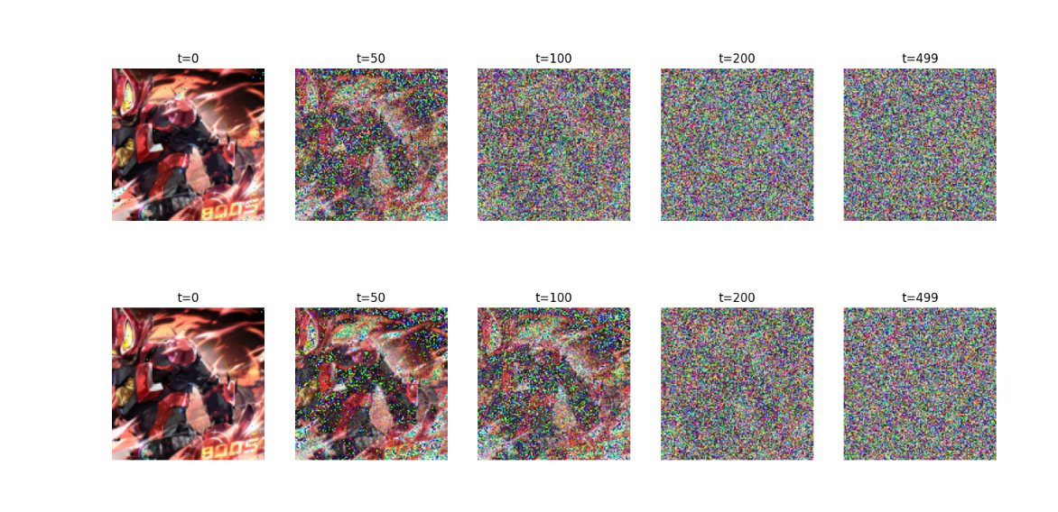
3、测试样例
1
2
3
4
5
6
7
8
9
10
11
12
13
14
15
16
17
18
19
20
21
22
23
24
25
26
27
28
29
| image_dir = "/home/student/lzp/1.Diffusion model/DIffusion model-myself/80bf302d92810c2b41.jpg"
image = Image.open(image_dir)
image_size = 128
transform = transforms.Compose([
transforms.Resize(image_size),
transforms.CenterCrop(image_size),
transforms.PILToTensor(),
transforms.ConvertImageDtype(torch.float),
transforms.Normalize(mean=[0.5, 0.5, 0.5], std=[0.5, 0.5, 0.5])
])
x_0 = transform(image).unsqueeze(0)
plt.figure(figsize=(16, 8))
for i in range(2):
if i == 0:
diffusion = GaussianDiffusion(timesteps=500, beta_name="linear")
else:
diffusion = GaussianDiffusion(timesteps=500, beta_name="cosine")
for idx, t in enumerate([0, 50, 100, 200, 499]):
x_noisy = diffusion.q_sample(x_0, t=torch.tensor([t]))
noisy_image = (x_noisy.squeeze().permute(1, 2, 0)+ 1) * 127.5
noisy_image = noisy_image.numpy().astype(np.uint8)
plt.subplot(2, 5, 1 + idx + 5*i)
plt.imshow(noisy_image)
plt.axis("off")
plt.title(f"t={t}")
plt.show()
|
img就是选择你想要加噪图像的地址,这里演示的是分别使用线性加噪以及余弦加噪的示例:
二、总结
本文介绍了扩散模型的加噪和去噪过程当中,一些公式如何用python语言去编写,也展示了线性加噪和余弦加噪的可视化。下回将会编写扩散模型是如何使用UNet预测噪声,以及是如何训练和采样。
